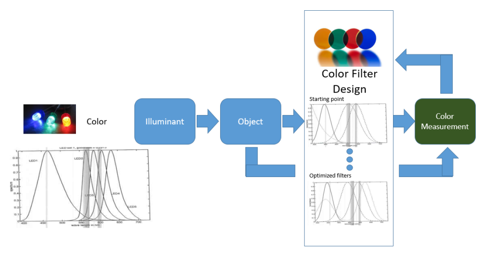
Figure 1: Generalized Diagram of “Color Filter Design for Multiple Illuminants and Detectors.
I am a very strange electrical engineer. I admit it. Unlike most EEs, I came from a Graduate School background in color image processing (a specialized subset of digital signal processing). I worked for Dr. H. J. Trussell at N.C. State; and it is because of him I did not turn into a pure networking guy. With color science; there is an appreciation to the emotional appeal of colors — and for the North Carolina textile industry — getting those colors right. Fast forward to today; and I bring a strong consideration for user perception and experience.
By the time I arrived in 1993, the textile industry in North Carolina had waned. Dr. Trussell was already making a leap into digital color science; a much needed area when you consider that basic color printers used to make Windows 95 freeze; affordable color digital monitors weren’t available en masse; and the first consumer digital cameras were just making it to marketplace.
The Problem We Were Trying to Solve
At this time, measuring color accurately was a very tedious process. To do it well, you needed to use a giant spectrophotometer – which in those days were large and expensive equipment.
The goal of my Master’s Thesis was to create a way to generate color filters that, when used with a set of a new (at that time) thing called LEDs, would accurately measure the color of an object. You can read my Master’s Thesis here. Figure 1 is a generalized visual for what is in the experiment.
The illuminants are fixed. We had 5 LEDs — but it could conceivably had been less or more. See Figure 2 – roughly Blue/Violet, Green, Yellow, Orange, and Red . We want to design 4 filters that would, colormetrically, give us the best prediction of color.
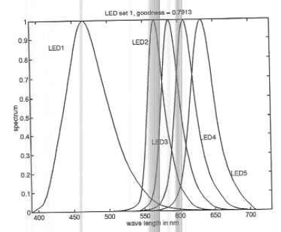
Figure 2: Input LEDs
The Intelligence in AI
As I mentioned before, my first encounter with neural networks as an Undergraduate at Georgia Tech — applied to predicting weather conditions. Very similar to that:
- The training set of illuminants and objects were well known spectrally in Table 3. We know the “inputs”; and we know what the “outputs” exactly.
- The curves for the filters could be modeled as Gaussian curves. Thus generalized version for the “weights” were capture in (4).
- There was an ability to calculate the colorimetric Goodness (ref. Vora) and thus error of a certain model.
But the similarity to a straight neural network ended there. Unlike a neural network, the Goodness calculation was a transform into a different space. And unlike the Cloud computing resources + AI libraries of today, I was limited by the computing power of 1994/1995. A back propagation based neural network wouldn’t have put me in a place to graduate anytime that decade.
The key to my thesis was the use of the Simplex algorithm. Dr. Trussell suggested this approach and straight forward as long as the filters were straight Gaussian shaped. But…what about filters that had multi-node Gaussians with different transferrance functions?
That is where I got creative. Figure 3 is the basic structure used. Program 1 can be thought of as “the Brains”. It was an executable that, in today’s terminology, is a form of Q-Learning / reinforcement learning. If we had reached an optimization point (min E) with the first filter types (we used four simple Gaussian shaped filters), it would save the filter set. Then it would adjust the type (ex. three simple Gaussian, and one 2-node Gaussian filter); and start again.
Program 2 can be thought of as “the Math Workhorse”. Program 2 taking on the heavy math calculations as well as executing the Simplex Algorithm. Program 1 would open Program 2 and add code for calculating V based on the filter # and filter types. Program 1 would then execute Matlab (a math application) that ran Program 2; which produced V, E and new filter parameters.
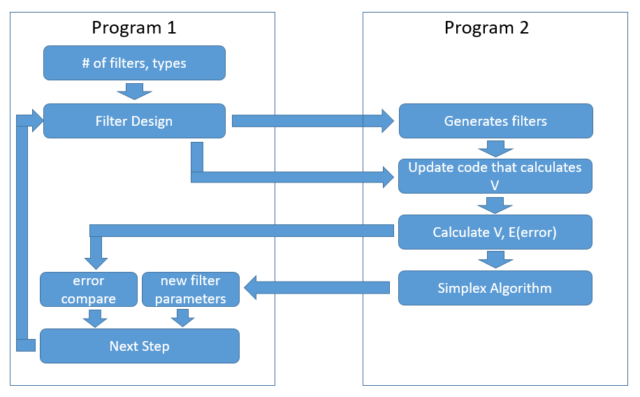
Figure 3: A Program that wrote another Program
Solve One Problem, Create Another
After the first several passes; I realized that Program 1 was still not optimized. Yes, I could get the best filter set of four normal Gaussians; and the best filter set for three normal + 1 two-node Gaussians. But in the end, we are looking at (transmittance levels)x (width of Gaussians)x(nodes)!*(Number of filters)! combination or 9 x 8 x 3! x 4! = 31,104 passes. Gah!!!
This is where another dose of creativity came in. In my second version of Program 1, I treated the transmittance level and nodes as just another parameter in the Simplex Algorithm. This is very similar to how they now use the concept of “fully connected” networks in Deep Q Learning and A3C; but at a smaller scale.
And…the new path ran it’s course. I hit the [Enter] key on Monday and got the results by Thursday. My program that wrote another program worked!!!
Looking At The Results 20+ years laters
Figure 4 shows the optimal 4 filters. The first three filters from the left look like wide-band mirrors of the color LEDs used – roughly Violet, Green, Yellow, and Orange. However, Filter 4 is the most interesting!!! The two node filter, is almost the same shape as a generic White LED. In other words, the most optimal energy to read is as close to reflective White.
I graduate in 1995, on-time for a 2 year Masters program. Looking back now, if the research would have continued; I wonder: “What are the minimal number of LEDs and filters (and their design) to still get the best color measurement results?” I am pretty sure Dr. Trussell or my old office mate, Dr. Guarav Sharma answered this years ago.
The Big Idea: If you look at the basic premise of this original problem; the mechanism is essentially the same for IR sensors and detectors in digital cameras and security cameras. Thanks Dr. Trussell for giving me a shot at working on this!!!
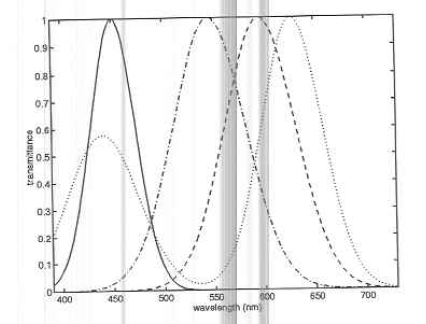
Figure 4: The Results
